COMBINING DATA FROM MULTIPLE SHEETS USING VLOOKUP

What is VLOOKUP?
VLOOKUP stands for 'Vertical Lookup' as it searches vertically through columns for values in multiple worksheets (or workbooks), allowing users to retrieve corresponding data efficiently.
The general syntax for using VLOOKUP is:

=VLOOKUP(lookup_value, sheet_name!table_array, col_index_num, [range_lookup])
lookup_value: This is the value you want to search for in the first column of the specified range. It is typically a cell reference from the current sheet (e.g., A2)
sheet_name!table_array: This is the source sheet name, followed by the range of cells that contains the data you want to search through in that sheet. For example, if your data is in Sheet2 and covers cells A1 to E100, it would be written as Sheet2!A1:E100.
col_index_num: This is the column number in the table array from which you want to retrieve the value. For example, if you want to return a value from the second column of the specified range, you would enter 2.
[range_lookup]: This is an optional argument to specify whether you want the formula to return an exact match (FALSE) or an approximate match (TRUE). It is best practice to use FALSE in most cases, especially when working with unique identifiers (like IDs or names), to ensure accurate results.
Now let’s practice how this works...
Imagine you are in charge of curating the graduating list for a university and to get the information needed, have to work with two (or maybe more) sheets in a workbook:
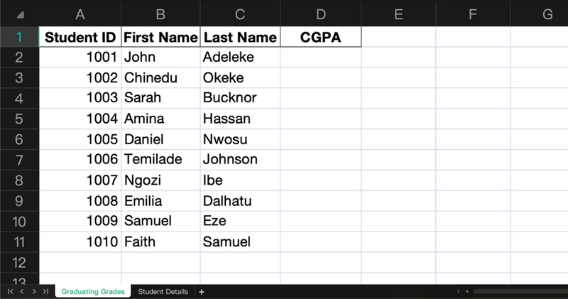
Sheet1 (Graduating Grades): Contains a list of student IDs and their names.

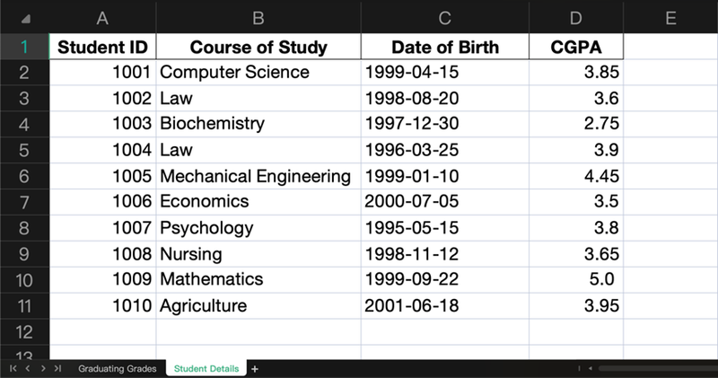
Sheet2 (Student Details): Contains student IDs, and other details including each student’s cumulative grade point average.

Your task is to populate the CGPA in Sheet1 (Graduating Grades) by pulling them from Sheet2 (Student Details) based on matching student IDs.
Here is a Step-by-Step Guide For Using VLOOKUP:
1. lookup_value: In Sheet1, column A contains the student IDs, which will be used as the lookup value. Let’s start with A2.
2. table_array: The data range in Sheet2, where the student ID is in the first column, and the CGPA is in another column. Suppose the range is from columns A to D, where:
- Column A has the student IDs,
- Column D has the CGPAs. The table array will be Sheet2!A:D.
3. col_index_num: Since the CGPA is in the fourth column (D) of Sheet2, the col_index_num will be 4.
4. range_lookup: To ensure you retrieve the exact match for the student ID, remember our best practice of using FALSE.
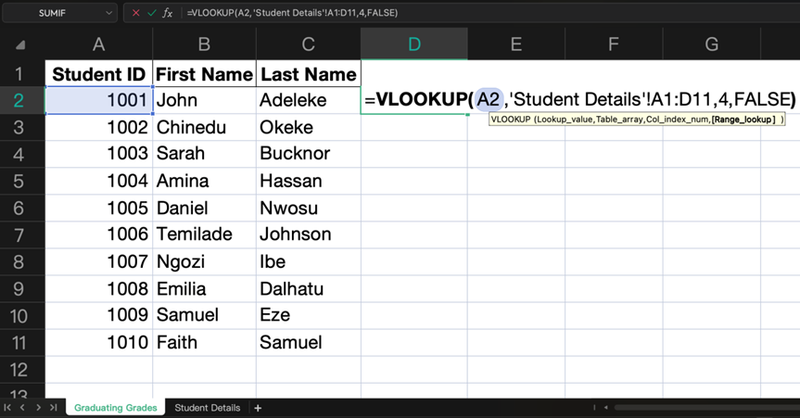
In Sheet1 (Graduating Grades), cell D2 (where you want the CGPA to appear), you will enter the following formula:
=VLOOKUP(A2,'Student Details'!A1:D11,4,FALSE)

Now, imagine this dataset is much larger — perhaps with thousands of rows. Instead of specifying a small range like A1:D11, you would expand the range to include all the relevant rows. It is more efficient to use a dynamic reference like A:D rather than specifying a fixed number of rows, to accommodate future expansion. When working with a growing dataset, using A:D tells Excel to look through the entire columns A to D, no matter how many new rows are continually added.
Our formula would then be:
=VLOOKUP(A2,'Student Details'!A:D,4,FALSE)
Using VLOOKUP Between Multiple Workbooks
VLOOKUP can also be used between separate workbooks. This feature is particularly useful when the data you need to retrieve is stored in a completely different file.
To perform a VLOOKUP between workbooks, you will need to reference both the workbook and the sheet where your data is located in your formula.
=VLOOKUP(lookup_value, [workbook_name]Sheet_name!range, col_index_num, [range_lookup])
If for instance, you want to pull the CGPA data from Workbook2, where they are stored in Sheet, with student IDs in column A and CGPAs in column C.
Below is what the syntax would look like:
=VLOOKUP(A2, '[Workbook2.xlsx]Sheet1'!A:C, 3, FALSE)

This formula will:
- Take the student ID from A2 in our current workbook.
- Look for that student ID in Workbook2, specifically in Sheet1, columns A to C.
- Return the CGPA from the third column (C) in Workbook2 where the exact match is found.
If the workbook you are referencing is closed, Excel will store the full file path in the formula, which may look like this:
=VLOOKUP(A2, '[C:\Users\YourName\Documents\Workbook2.xlsx]Sheet1'!A:C, 3, FALSE)
In this case, if the file location is changed, you will need to update the file path in the formula.
Conclusion
The VLOOKUP function is a powerful time-saving tool for data consolidation.
Unlike copying and pasting, using VLOOKUP allows your destination cells to automatically update whenever you change the information in the source tables.
However, while VLOOKUP is known for searching data vertically, it exclusively retrieves values from left to right. This limitation means that the lookup value must always be in the first column of the specified range.
For more complex data analysis or situations where you need to look up values to the left, other functions like INDEX and MATCH, or the more advanced XLOOKUP can be used for greater flexibility.
In summary, VLOOKUP is best suited for scenarios where the dataset is structured appropriately and unique identifiers are utilized. Mastering this function will enable you streamline your data analysis processes and improve your efficiency as a data analyst.
Author: Ayomikun Ojueromi
LinkedIn: https://www.linkedin.com/in/aojueromi/
