COMMON ADVANCE EXCEL FORMULAS FOR DAILY ANALYSIS

Below are some of the advance excel formulas that you can use to improve your analytical skills and make your work seamlessly easy.
- SUBSTITUTION
- DATA VALIDATION
- VLOOKUP
- XLOOKUP
- EXTRACT (YEAR, WEEKDAY, MONTH)
- COUNTIF
- SUMIF
- IFERROR
- CURRENT TIME
- INDEX & MATCH
Remember that you only learn by doing. So, always practice in other to improve your skills.
SUBSTITUTION: It is used to correct errors in Excel. When there is a need to update or modify a text string in a table or a dataset.
Formula is written as: =SUBSTITUTE(TEXT_COLUMN, OLD_TEXT, NEW_TEXT)
Always remember to include an apostrophe “” if you are going to key-in the text yourself without picking from the table.

In this instance, I have successfully changed Tiffany to TIMOTHY
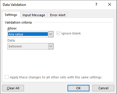
DATA VALIDATION: In Excel, you can decide the type of data that should be entered in a cell or the entire sheet. The process of doing that is what is known as data validation. Its purpose is to ensure an error free data, accuracy and consistence in form. You can also use it to create a drop-down list.
REMEMBER THAT YOU CAN ONLY LEARN BY PRACTICING
Steps:
Click on data from excel tab
Click on data validation

Make sure to try your hands on all the list in the above box.
VLOOKUP: This function is used to search values from the left part of a column and retrieve the searched value in the same row of a different column.

Lookup_value: This is the value you want to search for in the first row of the table.
Table_array: The cell range where what you intend to search for is. Don’t forget to include the first row of the table of better still, select the entire table.
Col_index_num: The column number of the value you want to retrieve. Remember the first column is number 1.
Range_lookup: Here you choose whether you want an approximate match or an exact match. It is advisable to pick exact match so it doesn’t mess your work up or give you a wrong answer.
COMBINATION OF DATA VALIDATION X VLOOKUP: Both functions can be used to summarize a table by using LIST on the drop-down of data validation table.
USE THIS LINK FOR A SHORT VIDEO: https://drive.google.com/file/d/1tFk9DgCXw8WLJuhNwYkyK_PJeWpo5irS/view?usp=sharing
XLOOKUP: Xlookup, unlike VLOOKUP and HLOOKUP, it is used to search and return values in a table without restrictions.
Vlookup searches only vertically, Hlookup searches only horizontally but XLOOKUP has no restriction. XLOOKUP is in the recent version of Excel as it cannot the found in 2019 and below version.

Charlie is the lookup value, A2:A4 is the lookup array, while B2:B4 is the return array.
EXTRACT: In Excel, we can separate the DAY, MONTH and YEAR from the DATE by using any of the extraction model.


COUNTIF: The countif function is used to count the values in a column if a specific term or condition is met.
If I want to count only the number of times that Apple appeared in a particular column or entire sheet, the formula becomes:
=COUNTIF(CELL_RANGE, “APPLE”)

To show the count of people that is aged above 35 years

SUMIF: Just like COUNTIF, SUMIF also sums up all the value that meets a specific condition.
To show the sum of salary that is above 80

B:B represents the salary column, while >80 is the condition.
IFERROR: This is used to handle errors in Excel. Usually, when we write wrong formulas, we get Errors in form of #N/A or #REF or #VALUE! Or as the case may be. Instead of these errors to appear, we can use the IFERROR formula to specify what we want it to return.

The above image would have returned error if the IFERROR formula wasn’t attached.

NB: You can notice that the IFERROR was used with a simple division and a complex vlookup function. So, the IFERROR formula can be used on its own or along with other easy or complex formulas.
CURRENT TIME: Excel has the ability to show what the current time and date is. All you have to do is use the formula NOW the open and closed bracket.
=NOW()

INDEX: The index formula is used to lookup data from a table or a range.


MATCH: While index returns the content of the search, MATCH returns the value in form of the position.

NB: while INDEX returned the content of the search in the cell (+AB), MATCH returned the POSITION in value (3)
INDEX & MATCH: This 2 can be combined to lookup values in a table. When searching for a value in a column but want to return the corresponding value in a different cell, a combination of both functions can then be used.

N.B: From the above formula, I returned the corresponding value of A5 in column B
Author: Obiwulu Chinyeaka David
LinkedIn: https://www.linkedin.com/in/chinyeaka-obiwulu-7b204a1a4/
Twitter: https://x.com/Oluwayeaka?t=gvo1yusDVkYzDPgqBO9Zog&s=09
