Unlocking the Power of INDEX MATCH: Real-World Use Case

The MATCH Function
MATCH belongs to the same to the same family as LOOKUP functions, albeit with more flexibility.
MATCH works by returning thee relative or exact position of an item in a range (image below).

The function takes 2 required arguments and 1 optional argument as demonstrated below.

lookup_value: the item we are interested in searching for.
lookup_array: where (the range) we would like to search either horizontally or vertically.
match_type : an optional argument that allows us to choose how we want the lookup_up to be searched, the available options are -1, 0, 1. While 1 is the default, setting the option as 1 returns the exact match of the value.
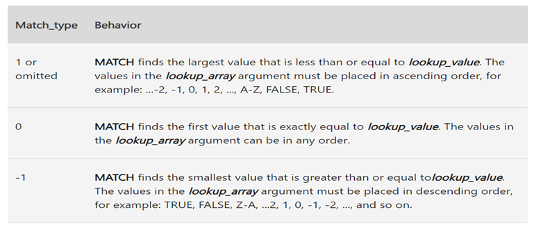
In summary, using the MATCH function is basically saying “Hey!, look into this place and return the position of this value within the place”
The INDEX Function
As in the image below, this function works by returning the data in a cell within a table after being specific with the position of the row and/or column.

Using the INDEX array or reference function could be likened to saying “hey! I know the address but I’m not sure who lives there, kindly find me their name”

Okay, that’s enough for an introduction, let’s get our hands busy!
INDEX-MATCH COMBINATION
I have these datasets in different tabs (as shown in the images below) and I have been assigned a task to create another variable called Rating using the Industry ratings tab as reference while ascertaining that the values correspond.
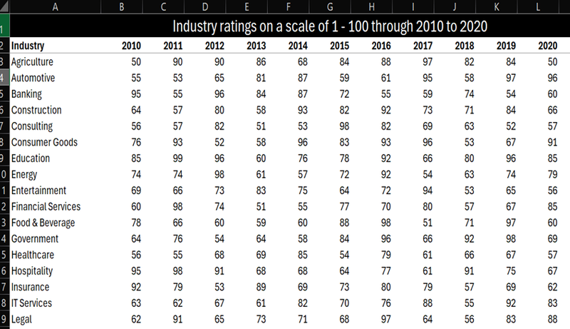
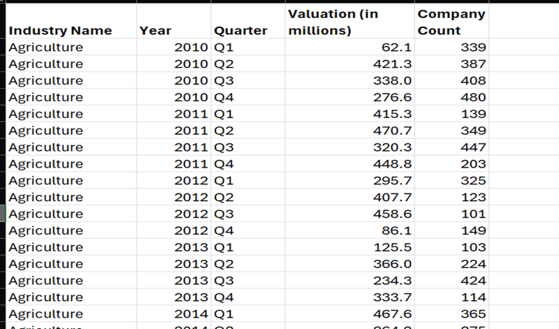
Firstly, let’s locate the row numbers and column numbers of year and Industry type respectively in the Industry Ratings tab.
Position of Industry using MATCH (row_num)


Position of year using MATCH (col_num)

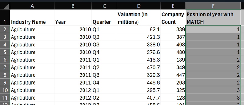
Now that we’ve located the exact position of the rows and columns, what’s left is to combine these formulae with INDEX in order to return the corresponding rating values in these identified positions.

As we can see in the syntax above, after the row_num and col_num have been defined, it’s easier to use INDEX function as we now only need to select the reference tab or array.
And we have this result.
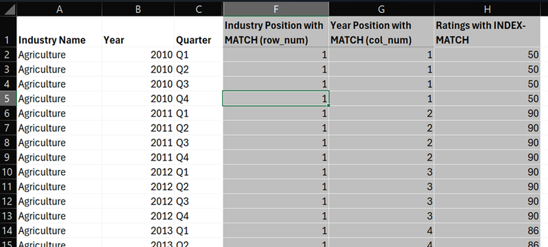
Going back to the Industry ratings tab, we could compare to see if our results are accurate as shown below.

This among many other ways, is how we can make good use of Excel functions to deliver accurate and insightful results.
One very helpful tip to keep in mind when working with multiple Excel functions is to break it down and start from the smallest/simplest before merging them to something more complex.
Thank you for reading
Taofeecoh Adesanu.
